

We made a short video about the project, which can be seen HERE.
The objective of this blog is to report on the progress of our project researching kelp aquaculture and to broaden awareness of integrated multi-trophic aquaculture systems. Our research will use a modeling approach to identify ideal site conditions for kelp-oyster aquaculture in Rhode Island. This model will help to determine the environmental feasibility of this kind of system in our local waters of Narragansett Bay and the south coast salt ponds. We are using this page as a forum for communication and to keep interested folks updated on the project activities and findings. We acknowledge support for this project from USDA National Institute of Food and Agriculture and NOAA Saltonstall-Kennedy.
We made a short video about the project, which can be seen HERE.

Since my last modeling update on this blog, I have made a combination of tiny steps and leaps of progress on understanding Dynamic Energy Budget (DEB) theory and in particular how it relates to photosynthetic organisms. I am using a DEB model to predict individual blade kelp growth through tracking the movement of mass from assimilation to use in maintenance, building new structure, or excretion.
We have had the basic structure and equations of the kelp DEB model since this past summer. The main modeling task I am working on currently is gathering data from the literature on parameters for the model. Parameters are fixed values in the equations such as maximum assimilation rate of nitrogen. This has proved to be quite a challenging process, because even though many papers have been published on sugar kelp, it is very infrequent that data is collected in the exact format needed for a particular parameter. Many parameters within the DEB model are too DEB specific to be directly related to literature values, so these will be fit to our field data within a logical range in comparison with an existing DEB model for phytoplankton (Lorena et al, 2010). I have spent a particularly large chunk of time trying to get an Arrhenius temperature, a marker of how temperature impacts metabolic rate, by compiling various metabolic rate data and converting it into a usable form. WebPlotDigitizer by Ankit Rohatgi has been a very valuable tool for gathering data from graphs in publications. In this process of thinking deeply about each parameter, guidance from our collaborator Dr. Romain Lavaud has been crucial. Romain has been able to re-direct me when I end up going down a particular parameter rabbit hole and clarify whether or not sources of data are reasonable references for this project.
Once I have as many parameters estimated with literature values as I can, we will start running the model in comparison to our field data to see how the DEB-specific parameters can be fit to provide a good fit of the model to the field data. Stay tuned!
Written by: Celeste Venolia

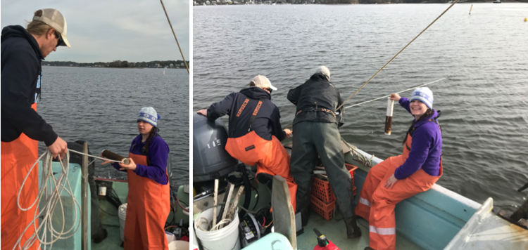
Russel Blank ties the seed line into the rope that kelp will be planted on while Dr. Lindsay Green-Gavrielidis holds the tube of kelp she grew. Photo Credit: Celeste Venolia.
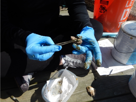
Cold temperatures have arrived and that means it is time to get the second year of kelp sporophytes planted out at the farms! Dr. Lindsay Green-Gavrielidis of the University of Rhode Island has been keeping a watchful eye over the young kelp sporophytes in the URI aquaria. This year, I was around to help with some of the reproductive tissue preparation in the fall. It was quite fun picking out the best pieces of reproductive tissue and getting to cut them out of the kelp blades for Lindsay to process them for eventual spore release. By the time the kelp sporophytes were ready to go in the water, the tubes with line wrapped around them looked like brown fuzzy caterpillars with all the kelps growing attached to the line. For a more detailed narrative of the nursery process check out Dr. Green-Gavrielidis’ post from year one of this blog.

Dr. Lindsay Green-Gavrielidis holds the tube of young kelp making sure that it feeds onto the line smoothly while Celeste Venolia keeps smooth tension on the rope. Photo Credit: Celeste Venolia.
Getting to plant the kelp out on the farms was very cool though at times nerve-wracking. The first task out at the farms was to make sure that the supporting gear was in place. The rope that the kelp is attached to is in the water between mooring balls. It is best to plant on a day without much wind, because with even a small current this rope can be hard to tension close to a straight line between the two mooring balls. Once it was time to plant and the kelp seed line was tied onto the rope, Lindsay and I got into a comfortable pattern of her holding the kelp tube and making sure the seed line fed smoothly onto the rope while I kept tension on the rope. Sometimes the boat would swing about a bit in the current, so the angle on the tensioning was quite a workout. During one of the later planting trips, I wrecked a pair of thick plastic work gloves. The friction between the rope and the gloves was so great that the rope ripped off some pieces of the glove. Once the kelp line was running out, the trick was to hold the rope in place, so that the seed line could be again tied into the rope and sensor rigs for irradiance and temperature data could be left out at the site. The nifty thing about kelp is that once it is in the water the farmers don’t have to do anything other than make sure the gear stays in place. The kelp thrives and grows quickly with the local conditions of light and nutrients.

Cedar Island Oysters growth over time at two different sites in Point Judith Pond. Photo Credit: Celeste Venolia.
In other in-the-field news, oyster growth as expected has slowed through the fall and now essentially stopped as oysters go dormant in the cold temps. They live off of resources gathered during the warm summer season. The tagging method we are using with PIT tags in epoxy and a PIT tag reader has performed well for the most part. Some oysters have lost their tags over time. Others died during the warmer months from ambiguous causes or from obvious causes like oyster drills, which are a common challenge for oyster farmers.
Written by: Celeste Venolia

Ocean model grid for Point Judith Pond and the surrounding waters generated by MS student Celeste Venolia using EASYGRID code in MATLAB.
I put energetics modelling work on hold for the latter part the fall semester (2018) to focus on getting oriented with Regional Ocean Modelling System (ROMS). ROMS is a grid-based primitive ocean equations hydrodynamic model that University of Rhode Island (URI) Associate Research Scientist Dave Ullman is working with for all the coastal waters of Rhode Island. For this aquaculture project, the goal is to predict the environmental variables across coastal RI needed to understand kelp and oyster growth. For example, for the kelp energetics model, we need a time series of dissolved inorganic nitrogen, total inorganic carbon, and irradiance. The reason that Dave started helping me learn ROMS is that in his bigger state-wide model the Saugatucket River is too small to be included in the set of rivers impacting the model. This absence matters for this aquaculture project because the Saugatucket River feeds into Point Judith Pond where two of our sites are located (Cedar Island Oysters).
This semester I am taking a great class at URI called Programming for Scientists with Professor Brice Loose, and a large part of this class is a final project where we utilize our coding skills in any scientific way that interests us. Brice decided to let me try to get as far as I could into learning how to run a small ROMS model for the Point Judith Pond area. The goal is to link this smaller model to the larger model that Dave is working on. A BIG thank you to Dave for all the time he has spent and continues to spend meeting with me to help me get oriented in ROMS world. Through meeting with Dave, I gained great appreciation for how much work goes into getting these models to run accurately. I would learn about a few file types and think I understand the whole picture and then be shocked the next week to discover that there were three more files to set up.
The main task that I have completed so far in ROMS world is figuring out how to generate a grid that ROMS can understand and run its equations along. There are multiple options in terms of programs that people have written to aid in grid generation, and I spent a bit of time working to download and consider different options. What ended up working for me is a code file in MATLAB called EASYGRID. Checkout the grid I created through the modification of this code (shown above)! We have the cells set at a pretty fine scale, so they almost look like a black fuzz across the image. More ROMS struggles to come!
Written by: Celeste Venolia

Dr. Romain Lavaud shows Celeste how his sea lettuce model runs in MATLAB. Photo credit: Austin Humphries
I started my Master’s thesis work with no mathematical modeling experience – just enthusiasm and a strong belief that anyone can learn anything they want to with the right resources and support.
The DEB Model
During Spring 2018, I spent a lot of time reading Dynamic Energy Budget (DEB) papers and some more general materials about the modelling process. DEB theory is a well-established way of modelling the flow of mass or energy through an organism from feeding or photosynthesizing to maintenance, growth, maturation, and reproduction. Just getting a handle on the underlying theory of this kind of model was challenging at first. Taking an online course about the basics of the theory helped orient me. Toward the end of Spring 2018, I worked to code an already published Eastern Oyster DEB model. I enjoyed the trial and error of problem solving code though there were definitely moments where I questioned whether the code would ever run. Getting the first model outputs that looked reasonable was a thrilling moment.
Canadian Excursion in the Name of Science!

Austin stands along the Petitcodiac River in Moncton, NB, Canada. The river has an impressive tidal bore and chocolatey-brown color. Photo credit: Celeste Venolia
During Summer 2018, I joined my graduate advisor Austin Humphries to travel to Moncton in Canada for a week to meet with Dr. Romain Lavaud who has been working on a DEB model for sea lettuce. We were super grateful that he took time to help us understand concepts and demonstrate how his code runs. Dr. Lavaud agreed to work with us on the sugar kelp DEB model, and we are excited to continue collaborating with him. At the end of the week, we got to be tourists, and I was pumped to see the tide change at the Bay of Fundy (a goal I set as a small ocean nerd). Through the rest of the summer and into the fall semester, I have been working to build a comprehensive list of model assumptions and potential parameter values from the literature for our sugar kelp model, while polishing my thesis proposal.

Celeste and Austin with Thomas Guyondet and Romain Lavaud for the obligatory group collaborator photo! Photo credit: some innocent bystander
We are collecting oyster growth data in order to have information to help fit energy-based oyster growth models for Rhode Island coastal waters. In the beginning of May, we went out to each of the farm sites and tagged 30 oysters and deployed temperature loggers.
Selecting the Tagging Method
Dr. Lindsay Green-Gavrielidis applies PIT tags to oysters with epoxy. Photo credit: Celeste Venolia
We had talked over a variety of potential tagging methods to track individuals over time and ended up going with PIT tags cemented to the oyster shells in epoxy because we were able to borrow at PIT tag reader from another lab at URI, and there is little risk of tags falling off the oysters. PIT stands for passive integrated transponder and the tags essentially function like barcodes. I recommend this piece from the journal Nature’s Knowledge Process if anyone wants to learn more about PIT tags. Working with the epoxy was like dealing with a swampy glue monster, but it made for very sturdy tags on the tops of the oysters.
The Art of Measuring an Oyster
We return to measure the oysters growth every month. The measurements we take are shell height and shell length. What height and length mean in relation to an oyster is not very intuitive. Shell height refers to the measurement from the umbo (the high point near the hinge of the two shells) to the farthest away point, and shell length refers to the widest distance roughly perpendicular to shell height. Shell height is the main measurement that most individual-based models in existence predict. The impression I have gotten talking to farmers is that rounder oysters are better for market, so it is also interesting to track shell length.

Left: Tagged oysters at Cedar Island Oysters at Point Judith Pond, RI. Right: MS student Celeste Venolia demonstrates how to measure oyster shell height. Photo credit: Lauren Josephs

Cindy West holds up a piece of her sugar kelp earlier in the season. Photo credit: Celeste Venolia
On April 22nd, I woke up nice and early to help Cindy and John West of Cedar Island Oyster farm harvest some of their sugar kelp lines. They had already spent a couple days harvesting, which was an impressive reminder of how much kelp they ended up growing. The harvest was an exhausting, but fun process. My height ended up being helpful as I would be the one to stand under the pulley as we all hoisted the new section of kelp line up onto the boat.
Kelp Biology Lesson

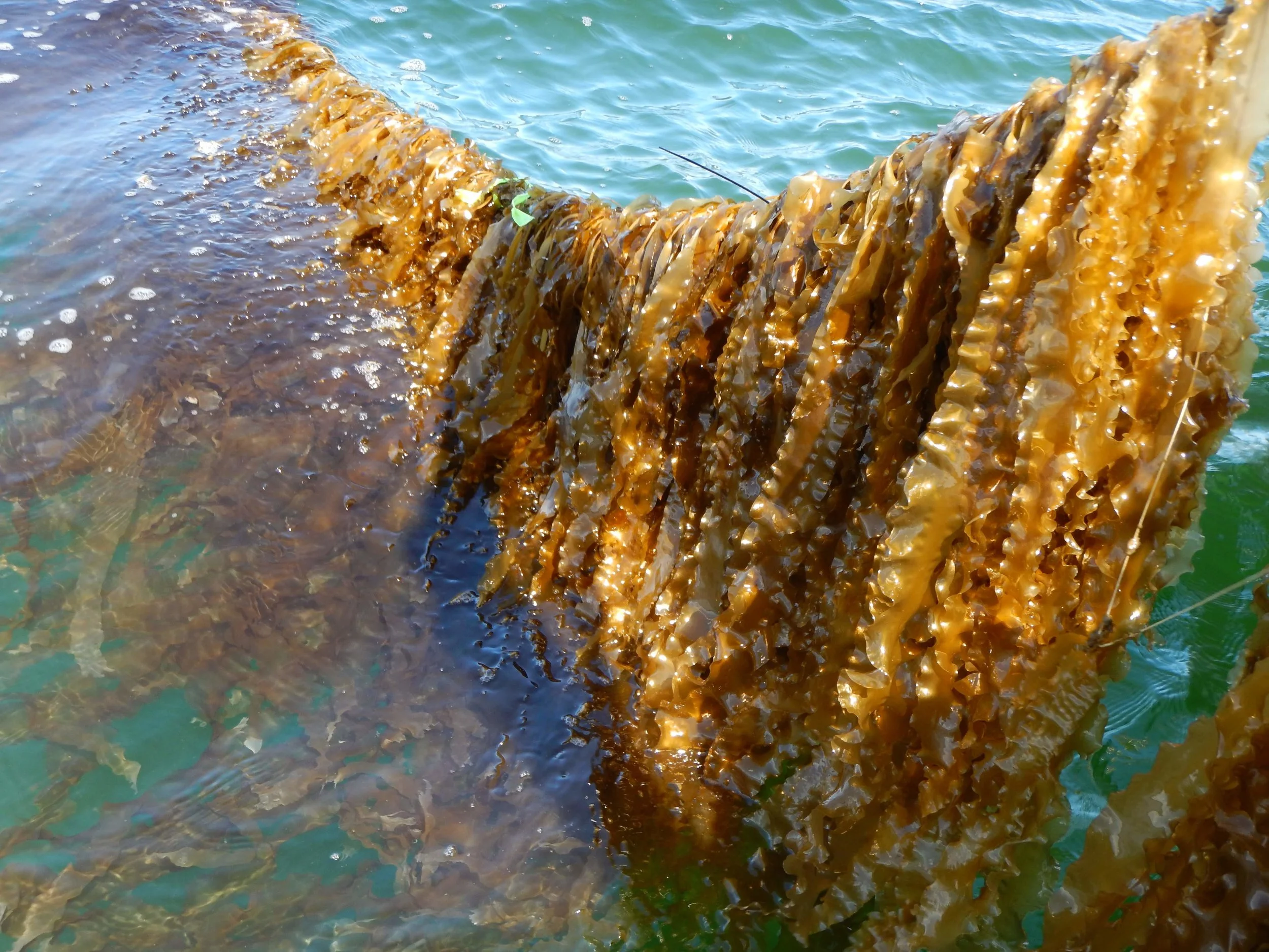
One of Cedar Island Oysters’ kelp lines underwater earlier in the season. The older tissue on this kelp is light in color. This portion will be cut off in the harvest process. Photo credit: Celeste Venolia
The kelp looked rather stunning hanging from the pulley. The ruffled blades hung together to form a luxurious golden brown curtain. From there we went about the process of cutting off the degraded tips of the kelp blades. Time for a bit of a kelp biology pause in the narrative. Kelps have a base structure called a holdfast that allows them to cling onto rocks in the wild or the lines they are seeded on in aquaculture systems. Connecting the holdfast and the main blade of the kelp is the stipe, a structure reminiscent of a stem. The main region of growth in the blade occurs near the stipe. As kelp grows and ages, the oldest tissue at the tip of the blade begins to be shed off. This older tissue is less desirable for human consumption. Trimmings of these degraded tissue were collected in one set of bags and the remaining blades were collected in another set of bags.
The Fate of the Kelp
Cindy and John sold their kelp to Sea Greens Farms, who turns the blades into kelp noodles. A processor also took the trimmings, but at a much lower rate per pound. I believe the trimmings end up being used as fertilizer on farms. The most physically challenging part of the day was after all the kelp was out of the water. We transported the heavy bags off the boat and into the truck, so they could be transported to refrigeration as quickly as possible.
Talking to Cindy at the end of this harvest, it became clear to me that for the kelp industry to have more staying power in Rhode Island the financial incentives for farmers need to be higher. Oysters are much more profitable for the amount of physical labor involved, given the way the kelp industry is currently structured and the high consumer demand for oysters. I hope that sooner rather than later kelp becomes more profitable for farmers, because it is a nutritious species with impressive yields that make it a good carbon sink in our oceans.
On April 21st, Dr. Lindsay Green-Gavrielidis, Professor Austin Humphries, and I joined Russ Blank of Rome Point Oysters to take some final growth measurements of kelp before the upcoming harvest. Since the lines were seeded and planted out at the farms, Lindsay has been going back every month to monitor the growth of the kelp, which is kept track of using a hole-punch as a reference point. This may sound like a strange way to monitor growth, but it is actually a tried and true method of kelp ecologists.
A Rome Point Oysters kelp line is pulled out of the water for growth measurements. Photo credit: Austin Humphries
The Hole-Punch Method
Hole punches are placed at a consistent 10 cm down the blade from the stipe (the stalk that supports the kelp blade). When we return a month later, the hole punch will have moved further away from the stipe along the blade and this can be measured to estimate elongation of the blade since it was hole punched.
Kelp Biomass Collection for Productivity Estimates

Celeste cuts kelp off the line for productivity estimates. Photo credit: Austin Humphries
On this particular trip, we collected individuals from each of the lines that had been hole-punched the previous month and hole punched a new set of individuals. Since this was our last visit out to the site before harvest, we also selected a 10 cm segment of rope on each line and collected all the kelp from these sections as a way of ultimately being able to estimate overall productivity. It was challenging to cut all of the holdfast pieces that had grown tangled together around the rope. Austin did a great job with the camera catching all the weird facing I made through this process. On some of the lines, many of the kelp blades were taller than me (I’m 6’1”). Lastly, a trip out on Russ’s farm wouldn’t be complete without a visit from one of his friendly seagulls who like to hang around on the front of the boat in case there are scraps.
Kelp Morphometrics and Nutrient Analysis
Back in the lab, Dr. Lindsay Green-Gavrielidis takes length and width measurements of the hole punched blades. Other individual kelp blades are dried on foil sheets. Once these individuals are dry they are ground up for carbon and nitrogen content analysis. You have to be careful with the mortar and pestle, because the dry kelp is quite brittle and prone to jumping out of the mortar. There is a lot you could analyze in these samples, but we will measure nitrogen and carbon content because nitrogen is the main nutrient limiting kelp growth and carbohydrates are made in the central process of photosynthesis. I will be using the kelp data collected to fit an individual energy-based growth model called a dynamic energy budget model.
In the fall of 2017, we established a sugar kelp nursery at the University of Rhode Island to produce “seed spools” of kelp to be planted at six different oyster aquaculture sites in Rhode Island. We followed methods for nursery cultivation of sugar kelp that were previously published in the “New England Seaweed Cultivation Manual: Nursery Systems” by Connecticut Sea Grant. This is the tale of the kelp as it progressed from spore to string to sea during the fall of 2017 and spring of 2018.
Wild Kelp Collection and Preparation

Reproductive kelp blades have a dark brown stripe, containing spores, down the middle. Photo credit: L. Green-Gavrielidis
On a late fall day, wild reproductive kelp was collected in Rhode Island by SCUBA diving. Reproductive kelps are easily recognized because they have a dark brown stripe down the middle— this is where the spores are. Kelp are reproductive throughout the year, but generally have a peak in reproduction in the spring and the fall. Since kelp farming occurs during the winter (in Rhode Island between November 1 and May 1), we collect wild kelp in the fall to raise in the nursery. After collection, tissue is cleaned in the lab, wrapped in damp paper towels, and placed in the fridge over night.
Spore Release and Seeding Spools
The next day, the tissue is taken out of the fridge and put into cool seawater. Over the course of the next hour of so, the seawater turns from crystal clear to milky brown as it fills with millions of microscopic, swimming kelp spores. After counting the spores with a microscope and diluting the seawater to the appropriate spore concentration, the spore solution is added to settling tubes. Settling tubes are large, closed PVC tubes that contain seawater and nutrients. Inside of the settling tubes are the seed spools. Seed spools are PVC pipes with nylon or cotton string carefully wrapped around them—this string is what the kelp spores will attach to and grow on. In order to encourage the spores to settle on the string, we place the settling tube with spore solution in a fridge, adjusted to 50F, in the dark for 24 hours.

On the left, reproductive kelp tissue (sorus) releasing spores and turning the water milky brown. On the right, our fridge outfitted with settling tubes. The seed spools and spore solution are added to the settling tubes, with sterile seawater and nutrients, and incubated in the dark for 24 hours. Photo credits: L. Green-Gavrielidis
Nursery Culture
The next day, the seed spools are ready to go to the nursery, where they will be for the next 6-8 weeks before returning to the sea. Over the course of the next three or so weeks, we will monitor the seed spools in the nursery, maintaining them at 50F. Kelps are temperate seaweeds and prefer cool temperatures. Every week, the spools will be moved to a new aquarium with clean seawater and nutrients. At the end of each week, we will increase the amount of light shining on to the spools. The gradual increase in light level serves as a natural signal to the kelp and encourages growth. When kelp spores initially settle on the seed string, they grow into microscopic (less than 10 cell!) male and female gametophytes. Over the course of several weeks, the light will encourage the gametophytes to develop and signal them to reproduce. Female gametophytes use hormones to attract sperm released from male gametophytes. After fertilization, a new golden-brown kelp sporophyte (think of the large kelp blades you see washed up on the beach) will grow out of the female gametophyte. When this process happens in the nursery, the bright white string on the seed spools begins to turn amber brown—a truly beautiful sight!

Seed spools that have been innoculated with kelp spores will appear white for approximately three weeks (left). After roughly three weeks of increasing light levels, the kelp gametophytes will reproduce and kelp sporophytes (or blades) will begin to grow, turning the seed spools golden brown (center). After an additional three weeks of growth, blades will be ready to plant on the farm (right). Photo credits: L. Green-Gavrielidis
Planting and Monitoring Kelp Lines
After roughly three more weeks, the kelp sporophytes will reach 1-5 mm in size and will be ready to plant on the farm. We wait until the water temperatures are below 60F, generally at the beginning of November, to plant the kelp lines. In 2017, we planted our first kelp lines on November 1 at all of our farm sites. Planting kelp lines is a fairly quick process because of the design of the seed spool. Once we are on the farm, we take a thick line, called the longline, that will support the kelp as they grow, and put it through the middle of the PVC seed spool. We then take the end of the thin kelp line and splice it through the longline, securing the end with several knots. At this point, we simply back the boat up at a slow pace and watch as the kelp line wraps around the longline. When we reach the other end, we secure the kelp line in place with some additional knots.
Austin and Lindsay Green-Gavrielidis work with oyster and kelp farmer, Cindy West of Moonstone Oysters to plant kelp in November 2017. Photo credits: Emma Ferrante

By mid-January, kelp on our Rome Point farm was reaching 3 feet in length! Photo credit: L. Green-Gavrielidis
After the line is seeded, it’s secured about 3 feet below the water surface. Putting the line below the surface protects it from any ice that may form during the winter months and from high-energy waves on the surface. Once the line is secure, the hard work is done. Now, over the process of 5-6 months, we will monitor the kelp growth. Every few weeks, we visit the farms to check the lines. Samples of kelp are collected to measure how much carbon and nitrogen they have in their tissues—a measurement of how suitable the site is for kelp farming and a measurement of how much carbon the kelp is sequestering. We also determine the growth rate of kelp blades using a hole punch. Kelp grown from the bottom of the blade, so we can use a hole punch to mark a spot and measure how far the hole moves over time!
Late December in Rhode Island was very cold, but by mid January we had at least 12” of growth on most of our lines, with some already reaching 3 feet in length. As the day-length increases and water temperatures rise, the kelp will continue to increase its growth rate. In the late spring, our kelp will begin to double in size every couple of weeks. By harvest time, which happens at the end of April, we expect kelp on most of the farms was between 6 and 9 feet long!

Dr. Lindsay Green-Gavrielidis
Co-PI Dr. Lindsay Green-Gavrielidis is a Postdoctoral Researcher in the Thornber Lab at URI. She has expertise in seaweed nursery set-up and cultivation systems. She has conducted research on aquaculture of several economically important seaweeds and was the co-author of a publicly available manual on how to set-up a nursery system for four species of seaweeds, including sugar kelp (Redmond et al., 2014). Dr. Green-Gavrielidis will be responsible for establishing and maintaining the kelp nursery and executing field experiments. Dr. Green-Gavrielidis will also assist in the workshops. Read more about Lindsay’s work here on her website.

Dr. Carol Thornber
Co-PI Dr. Carol Thornber is Associate Dean of Research in the College of the Environment and Life Sciences and a Professor at URI with extensive experience in seaweed ecology. Dr. Thornber will assist in the establishment of the kelp nursery provide seaweed expertise as needed. Read more about Dr. Thornber’s work on her lab website here.

Dr. Chris Kincaid

Dr. Dave Ullman
Co-PIs Drs. Kincaid and Ullman maintain both the Narragansett Bay Regional Ocean Modeling System (ROMS) model and the Coastal Hydrodynamics Supercomputer Cluster on which the model runs (located at URI). They are working on the development of the coupled hydrodynamic-biogeochemical model for Narragansett Bay and a few of the focal coastal salt ponds (Pt. Judith Pond). Check out more of Dr. Kincaid’s work here, and Dr. Ullman here.

MS student Celeste Venolia
MS student Celeste Venolia started working on the project in January 2018. She is working on the Dynamic Energy Budget model for kelp, as well as how this gets coupled to the hydrodynamic-biogeochemical model. When she isn’t coding in Matlab, R, or Python, she is learning lots about field and lab techniques from Dr. Green-Gavrielidis. More on Celeste can be found here.

Dr. Austin Humphries
PI Dr. Austin Humphries is trying to keep everything running smoothly.
None of this work would be possible without the generous help and collaboration of the Rhode Island oyster farmers (and now kelp farmers!). We are grateful for their time, patience, and willingness to work together on all aspects of this research project. They inspire us to do better work to help the local sustainable seafood industry thrive.
Additionally, we are working with Dr. Autumn Oczkowski at the EPA Atlantic Ecology Division, Bren Smith of GreenWave, and Dale Leavitt of Roger Williams University.
We are grateful for the NOAA Saltonstall-Kennedy (award #17GAR008) program for funding this work. The project period is 2 years, from Sept 2017 to 2019. Stay tuned for more information!